Branch-and-Price (BNP) Solver |

Contents
The Branch-and-Price Solver box on the Integer Solver tab:
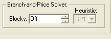
contains two parameters - Blocks and Heuristic - for controlling the branch-and-price (BNP) solver. The BNP solver is a mixed integer programming solver for solving models with block structures like the following:
Minimize: Σ c(k) * x(k)
Subject To:
Σ A(k) * x(k) = d (linking constraints)
x(k) in X(k), for all k (decomposition structure)
where d, c(k) and x(k) are vectors and A(k) is a matrix with appropriate dimensions. x(k) contains decision variables and X(k) denotes a linear feasible domain for x(k).
The BNP solver is a hybrid of branch-and-bound, column generation, and Lagrangean relaxation methods. It can help to find either the optimal solution or a better lower bound (the Lagrangean bound) for a minimization problem. Based on the decomposition structure, the solver divides the original problem into several subproblems, or blocks, and solves them (almost) independently, exploiting parallel processing if multiple cores are available.
BNP may perform better than the default MIP solver if: a) the number of linking constraints is small, b) the number of blocks is large and they are of approximately the same size, and c) the number of available processors (or cores) is large, e.g., 4 or more. Also, there may be some models for which BNP finds a good solution and good bound more quickly than the default MIP algorithm, although it may take longer to prove optimality.
The Blocks option for the BNP solver controls the number of subproblems, or blocks, that the model will be partitioned into. Possible setting for the Blocks parameter are:
| • | Row Names - Row names are constructed in such a way as to specify each row's block (an example is given below). |
| • | Off - This will disable the BNP solver, in which case, the standard MIP solver will be used to solve all mixed integer linear programs. |
| • | Specified - The user explicitly specifies each row's block using the @BLOCKROW function. |
| • | N - A positive integer, greater-than-or-equal-to 2, indicating the number of independent blocks to try and partition the model into via one of the graph partitioning algorithms provided by LINGO. The actual heuristic used is chosen with the Heuristic parameter. |
The default setting for Blocks is Off, i.e., the BNP solver will not be used on integer programming models.
The Block Heuristic parameter controls the heuristic used to partition the model into blocks. You may currently select from two graph partitioning algorithms named simply GP1 and GP2, with the default setting being GP1.
As an example, consider the following model:
MIN = x1 + x2 + x3 + x4 + x5 + x6;
[c1] x1 + x2 + x3 + x4 + x5 + x6 >=3; !linking constraint;
[c2] x1 + x2 <=1; !block 1;
[c3] x2 + x3 <=1; !block 1;
[c4] x4 + x5 + x6 <=2; !block 2;
[c5] x4 + x6 <=1; !block 2;
@bin( x1); @bin( x2); @bin( x3);
@bin( x4); @bin( x5); @bin( x6);
The above model has six variables and five constraints. Constraint 1 will be the only linking constraint, with linking constraints referred to as being in block 0. Constraints 2 and 3 constitute the first independent subproblem, or block 1. Constraints 4 and 5 form block 2. Thus, for this particular model, you would want to set the Blocks parameter to be 2, corresponding to the two independent subproblem blocks. For the partitioning heuristic, you may choose either GP1 or GP2. When we solve this model, note that the beginning of the solution report returned by LINGO contains the following information:
Global optimal solution found.
Objective value: 3.000000
Objective bound: 3.000000
Infeasibilities: 0.000000
Extended solver steps: 0
Total solver iterations: 14
Number of branch-and-price blocks: 2
The interesting feature to note is the line:
Number of branch-and-price blocks: 2
indicating that LINGO partitioned the model in to two independent blocks and invoked the BNP solver.
| Note: | Note that in some cases the number of blocks listed in the solution report may be less than the number of blocks requested. This occurs when the partitioning heuristic is unable to find a partition with the full number of desired blocks. |
| Note: | The BNP solver can run the independent subproblems on separate threads to improve performance. So, if your machine has multiple cores, be sure to set the thread limit to at least the number of blocks. Refer to the Threads parameter on the General Solver Tab, discussed above. For this particular small example with its two independent blocks, you'd want to set the thread limit to at least 2. |
The graph partitioning algorithms provided by LINGO can generally determine good partitioning schemes, however, for larger models, they may not be able to determine an optimal partitioning. In this case, you may prefer to explicitly specify a model's block structure. LINGO provides two ways to do this by either a) specifying the block structure as part of a model's row names, or b) specifying the block structure using the @BLOCKROW function. Examples of both follow.
To specify a row's block using its row name, you should begin the row name with the string "BNP_N", where N is the row's block number. The block number should be some non-negative integer, with a value of 0 indicating that the row belongs to the set of linking constraints. For example, using the model above, we could have specified the block structure in the row names as follows:
MIN = x1 + x2 + x3 + x4 + x5 + x6;
[bnp_0_c1] x1 + x2 + x3 + x4 + x5 + x6 >=3; !linking constraint;
[bnp_1_c2] x1 + x2 <=1; !block 1;
[bnp_1_c3] x2 + x3 <=1; !block 1;
[bnp_2_c4] x4 + x5 + x6 <=2; !block 2;
[bnp_2_c5] x4 + x6 <=1; !block 2;
@bin( x1); @bin( x2); @bin( x3);
@bin( x4); @bin( x5); @bin( x6);
You will also need to select the Row Names option for the Blocks parameter. When specifying block structure in row names, the Heuristic parameter is not relevant and will be grayed out.
Alternatively, you could use the @BLOCKROW( BLOCK_NUMBER, ROW_NAME) function to specify block structure. Again, using our same sample model, we would enter:
MIN = x1 + x2 + x3 + x4 + x5 + x6;
[c1] x1 + x2 + x3 + x4 + x5 + x6 >=3; !linking constraint;
[c2] x1 + x2 <=1; !block 1;
[c3] x2 + x3 <=1; !block 1;
[c4] x4 + x5 + x6 <=2; !block 2;
[c5] x4 + x6 <=1; !block 2;
@bin( x1); @bin( x2); @bin( x3);
@bin( x4); @bin( x5); @bin( x6);
@blockrow( 0, c1);
@blockrow( 1, c2);
@blockrow( 1, c3);
@blockrow( 2, c4);
@blockrow( 2, c5);
In this case, you will need to select the Specified option for the Blocks parameter. When specifying block structure via @BLOCKROW, the Heuristic parameter is not relevant and will be grayed out.