Local Optima vs. Global Optima

Contents
When LINGO finds a solution to a linear optimization model, it is the definitive best solution-we say it is the global optimum. A globally optimal solution is a feasible solution with an objective value that is as good or better than all other feasible solutions to the model. The ability to obtain a globally optimal solution is attributable to certain properties of linear models.
This is not the case for nonlinear optimization. Nonlinear optimization models may have several solutions that are locally optimal. All gradient based nonlinear solvers converge to a locally optimal point (i.e., a solution for which no better feasible solutions can be found in the immediate neighborhood of the given solution). Additional local optimal points may exist some distance away from the current solution. These additional locally optimal points may have objective values substantially better than the solver's current local optimum. Thus, when a nonlinear model is solved, we say the solution is merely a local optimum. The user should be aware that other local optimums may, or may not, exist with better objective values. Conditions may exist where you may be assured that a local optimum is in fact a global optimum. See the Convexity section below for more information.
Consider the following small nonlinear model involving the highly nonlinear cosine function:
MIN = X * @COS( 3.1416 * X);
X < 6;
The following graph shows a plot of the objective function for values of X between 0 and 6. If you're searching for a minimum, there are local optimal points at X values of 0, 1.09, 3.03, and 5.02 in the "valleys." The global optimum for this problem is at X = 5.02, because it is the lowest feasible valley.
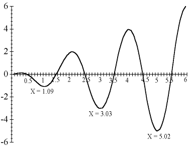
Graph of X * @COS( 3.1416 * X)
Imagine the graph as a series of hills. You're searching in the dark for the minimum or lowest elevation. If you are at X = 2.5, every step towards 2 takes you uphill and every step towards 3 takes you downhill. Therefore, you move towards 3 in your search for the lowest point. You'll continue to move in that direction as long as it leads to lower ground.
When you reach X=3.03, you'll notice a small flat area (slope is equal to zero). Continuing begins to lead uphill and retreating leads up the hill you just came down. You're in a valley, the lowest point in the immediate neighborhood--a local optimum. However, is it the lowest possible point? In the dark, you are unable to answer this question with certainty.
LINGO lets you enter initial values for variables (i.e., the point from which LINGO begins its search) using an INIT section. A different local optimum may be reached when a model is solved with different initial values for X. In this example, one might imagine that starting at a value of X=6 would lead to the global optimum at X=5.02. Unfortunately, this is not guaranteed, because LINGO approximates the true underlying nonlinear functions using linear and/or quadratic functions. In the early stages of solving the model, these approximations can be somewhat rough in nature. Therefore, the solver can be sent off to distant points, effectively passing over nearby local optimums to the true, underlying model.
When "good" initial values for the variables are known, you should input these values in an INIT section. Additionally, you may want to use the @BND function to bound the variables within a reasonable neighborhood of the starting point. When you have no idea what the optimal solution to your model is, you may find that observing the results of solving the model several times with different initial values can help you find the best solution.
LINGO has several optional strategies to help overcome the problem of stalling at local optimal points. The global solver employs branch-and-bound methods to break a model down into many convex sub-regions. LINGO also has a multistart feature that restarts the nonlinear solver from a number of intelligently generated points. This allows the solver to find a number of locally optimal points and report the best one found. Finally, LINGO can automatically linearize a number of nonlinear relationships through the addition of constraints and integer variables so that the transformed linear model is mathematically equivalent to the original nonlinear model. Keep in mind, however, that each of these strategies will require additional computation time. Thus, whenever possible, you are always better off formulating models to be convex so that they contain a single extreme point.