Piecewise Linear Example - Type SOS2 Set

Contents
As we mentioned above, SOS2 sets are particularly useful for implementing piecewise-linear functions. Many cost curves exhibit the piecewise-linear property. For example, suppose we want to model the following cost function, where cost is a piecewise-linear function of volume, X:
Piecewise-Linear Function Example
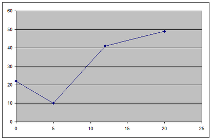
The breakpoints of the curve lie at the following points: (0,22), (5,10), (12,41) and (20,49).
The following sample model, SOSPIECE.LG4, uses a Type 2 SOS set to model this piecewise-linear function using what is referred to as the lambda method:
MODEL:
! Demonstrates the lambda method for
representing arbitrary, piecewise-linear
curves using an SOS2 set;
! See "Optimization Modeling with Lingo",
Section 11.2.7;
SETS:
! 4 breakpoints in this example;
B /1..4/: W, U, V;
ENDSETS
DATA:
! total cost at the breakpoints;
V = 22 10 41 49;
! the breakpoints;
U = 0 5 12 20;
ENDDATA
! set x to any value in interval--the cost
variable will automatically be set to the
correct total cost;
X = 8.5;
! calculate total cost;
COST = @SUM( B( i): V( i) * W( i));
! force the weights (w);
X = @SUM( B( I): U( I) * W( i));
!weights must sum to 1;
@SUM( B( I): W( I)) = 1;
! the weights are SOS2: at most two adjacent
weights can be nonzero;
@FOR( B( I): @SOS2( 'SOS2_SET', W( I)));
END
Model: SOSPIECE
We defined an attribute, W, whose members act as weights, placing us on an particular segment of the curve. For example, if W(2)=W(3)=0.5, then we are exactly halfway between the second and third breakpoints : (5,10) and (12,41), i.e., at point (8.5,25.5). In the case where we lie exactly on a breakpoint, then only one of the W(i) will be nonzero and equal to 1.
For this strategy to work correctly, only two, at most, of the W(i) may be nonzero, and they must be adjacent. As you recall, this is the definition of an SOS2 set, which we create at the end of the model with the expression:
! the weights are SOS2: at most two adjacent
weights can be nonzero;
@FOR( B( I): @SOS2( 'SOS2_SET', W( I)));
In particular, each weight W(i) is a member of the Type SOS2 set titled SOS2_SET.
For this particular example, we have chosen to pick an x-value and then let LINGO compute the corresponding y-value, or cost. Running, the model, as predicted, we see that for an X value of 8.5, total cost is 25.5:
Variable Value
X 8.500000
COST 25.50000
W( 1) 0.000000
W( 2) 0.5000000
W( 3) 0.5000000
W( 4) 0.000000
Solution to SOSPIECE
In addition to allowing the solver to work more efficiently, SOS sets also help to reduce the number of variables and constraints in your model. In this particular example, had we not had the SOS2 capability, we would have needed to add an additional 0/1 attribute, Z, and the following expressions to the model:
! Here's what we eliminated by using @sos2:
! Can be on only one line segment at a time;
w( 1) <= z( 1); w( @size( b)) <= z( @size( b));
@for( b( i) | i #gt# 1 #and# i #lt# @size( b):
w( i) <= z( i) + z( i + 1)
);
@sum( b( i): z( i)) = 1;
@for( b( i): @bin( z( i)));
| Note: | It may seem that piecewise linearity could be implemented in a more straightforward manner through the use of nested @IF functions. Certainly, the @IF approach would be more natural than the lambda method presented here. However, @IF functions would add discontinuous nonlinearities to this model. This is something to try and avoid, in that such functions are notoriously difficult to solve to global optimality. In the approach used above, we have maintained linearity, which allows LINGO to use its faster, linear solvers, and converge to a globally optimal solution. |