The Solution

Contents
The entire formulation and excerpts from the solution appear below.
MODEL:
SETS:
PERIODS: OBSERVED, PREDICT, ERROR;
QUARTERS: SEASFAC;
ENDSETS
DATA:
PERIODS = P1..P8;
QUARTERS = Q1..Q4;
OBSERVED = 10 14 12 19 14 21 19 26;
ENDDATA
MIN = @SUM( PERIODS: ERROR ^ 2);
@FOR( PERIODS: ERROR =
PREDICT - OBSERVED);
@FOR( PERIODS( P): PREDICT( P) =
SEASFAC( @WRAP( P, 4))
* ( BASE + P * TREND));
@SUM( QUARTERS: SEASFAC) = 4;
@FOR( PERIODS: @FREE( ERROR);
@BND( -1000, ERROR, 1000));
END
Model: SHADES
Local optimal solution found.
Objective value: 1.822561
Infeasibilities: 0.000000
Total solver iterations: 25
Elapsed runtime seconds: 0.05
Variable Value
BASE 9.718878
TREND 1.553017
OBSERVED( P1) 10.00000
OBSERVED( P2) 14.00000
OBSERVED( P3) 12.00000
OBSERVED( P4) 19.00000
OBSERVED( P5) 14.00000
OBSERVED( P6) 21.00000
OBSERVED( P7) 19.00000
OBSERVED( P8) 26.00000
PREDICT( P1) 9.311820
PREDICT( P2) 14.10136
PREDICT( P3) 12.85213
PREDICT( P4) 18.80620
PREDICT( P5) 14.44367
PREDICT( P6) 20.93171
PREDICT( P7) 18.40496
PREDICT( P8) 26.13943
ERROR( P1) -0.6881796
ERROR( P2) 0.1013638
ERROR( P3) 0.8521268
ERROR( P4) -0.1938024
ERROR( P5) 0.4436688
ERROR( P6) -0.6828722E-01
ERROR( P7) -0.5950374
ERROR( P8) 0.1394325
SEASFAC( Q1) 0.8261096
SEASFAC( Q2) 1.099529
SEASFAC( Q3) 0.8938789
SEASFAC( Q4) 1.180482
Solution to SHADES
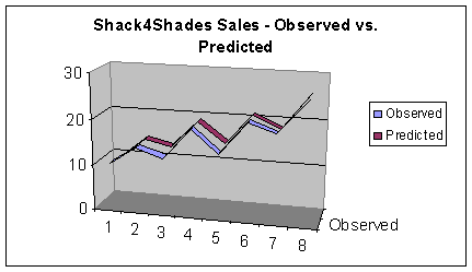
The solution is: TREND, 1.55; BASE, 9.72. The four seasonal factors are .826, 1.01, .894, and 1.18. The spring quarter seasonal factor is .826. In other words, spring sales are 82.6% of the average. The trend of 1.55 means, after the effects of season are taken into account, sales are increasing at an average rate of 1,550 sunglasses per quarter. As one would expect, a good portion of the error terms are negative, so it was crucial to use the @FREE function to remove the default lower bound of zero on ERROR.
Our computed function offers a very good fit to the historical data as the following graph illustrates:
Using this function, we can compute the forecast for sales for the upcoming quarter (quarter 9). Doing so gives:
Predicted_Sales( 9) = Seasonal_Factor( 1) * ( Base + Trend * 9)
= 0.826 * ( 9.72 + 1.55 * 9)
= 19.55
Given this, inventory levels should be brought to a level sufficient to support an anticipated sales level of around 19,550 pairs of sunglasses.